Evolutionary algorithms is a concept I first came across at University as a technique for solving optimisation problems, inspired by real-life biological evolution. For a final-year project, I was exploring possible ways in which you could reconstruct a shredded document from scanned images of its shredded pieces. The main issue with any algorithm is the complexity of the number of potential configurations of the pieces. For example, even if a single page was strip shredded (i.e. not cross cut) into just ten strips, then there would be 10 factorial possible configurations, i.e. 3,628,800. A typical shredder that cuts 6mm strips will produce 35 strips from a piece of A4, therefore 35 factorial equals 10,333,147,966,386,144,929,666,651,337,523,200,000,000 possible configurations to consider.
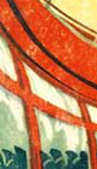
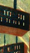
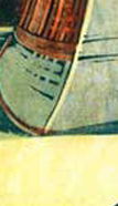
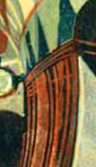
I thought I would revisit this concept many years later, and tackle cross cuts as well, and see how much of it I remembered. Instead of actually shredding and scanning paper, I just cropped an image I liked into 18 (3 x 6) pieces, and used the algorithm to reconstruct the image. For now, at least, I’ve allowed this algorithm to know that the solution is configured in 3 rows of 6 pieces, and all the images are already the correct way up. Here are the images:






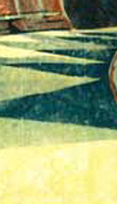

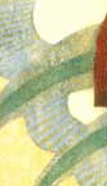
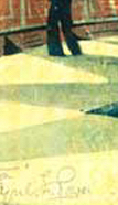


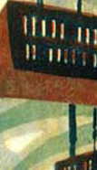

Here is the basic concept of evolutionary algorithms, courtesy of Wikipedia. Under each step, in blue, I indicate how this was implemented in this case:
Implementation
Step One: Generate the initial population of individuals randomly. (First generation.)
I started by generating 100 random solutions to the problem, i.e. completely random ordering of the pieces. I’ve made the population size easily changeable below so that we can see how it affects the performance of the algorithm.
Step Two: Repeat the following regenerational steps until termination:
• Evaluate the fitness of each individual in the population (time limit, sufficient fitness achieved, etc.).
The fitness of each solution is an overall measure of how similar the pieces are at the edges they share with their neighbours. This is calculated by converting the pixels on the edge into a greyscale value and totalling the differences along all adjacent pieces. Therefore, we are ultimately looking for a solution that produces the lowest difference/fitness value.
• Select the fittest individuals for reproduction. (Parents.)
This was just a case of sorting the population by fitness value and selecting the top performers. In our case, I selected the top 50%.
• Breed new individuals through crossover and mutation operations to give birth to offspring.
The idea here is to combine two solutions together in the hope that the offspring end up being a better solution. I have chosen to take a randomly sized rectangular selection of pieces from one solution and place it in a new random position in another solution, and the displaced pieces are then rearranged into the other part of the solution. Mutations, on the otherhand, occur within a single solution (i.e not a combination of two solutions) and in our case this could be the switching of two random pieces.
• Replace the least-fit individuals of the population with new individuals.
The worst performing individuals in our sorted population were removed and replaced by our newly bred individuals. The cycle then repeats indefinitely.
Outcomes
With each generation you are hoping that the newly bred individuals will provide a better solution than the ones that they are replacing and therefore the overall average fitness of population increases as you move towards the optimum solution.
As you may see in the simulation below, it is not guaranteed that the optimal solution is found. Sometimes it will find a good solution but be unable to be breed into a better one in one step despite there being a better one existing. In other words, it has converged on a local minima/maxima (i.e. not the global one), and the solution will have to get worse before it can get better, which it can’t do. This is a sign that the crossover or mutation techniques might not be sufficient to produce the best offspring.
In the simulation below, I have, for demonstration purposes, programmed it to stop when the correct solution is reached, but in reality, you would not necessary know if a solution was optimal. Instead, you could either run the simulation for a set number of generations, or stop it if no further progress has been made after a certain time.
Note, due to limitations of screen space, this simulation should ideally be viewed on a desktop machine.